Project 09

Three systems in Simulink.

Block diagram models of three dynamic systems, each driven from a MATLAB script that sets the parameters, runs the model and plots the response — a moving iron transducer, a DC shunt motor under load, and an inverted pendulum.

Three Simulink scopes showing motor speed, armature current and field current under a 1000 Nm load — Speed, armature current and field current at 1000 Nm.

Moving iron transducer

Force against a spring

A coil pulls an iron armature against a spring and damper. With no external force the armature settles at about 0.00295 m — the magnetic pull is tiny next to a 2500 N/m spring.

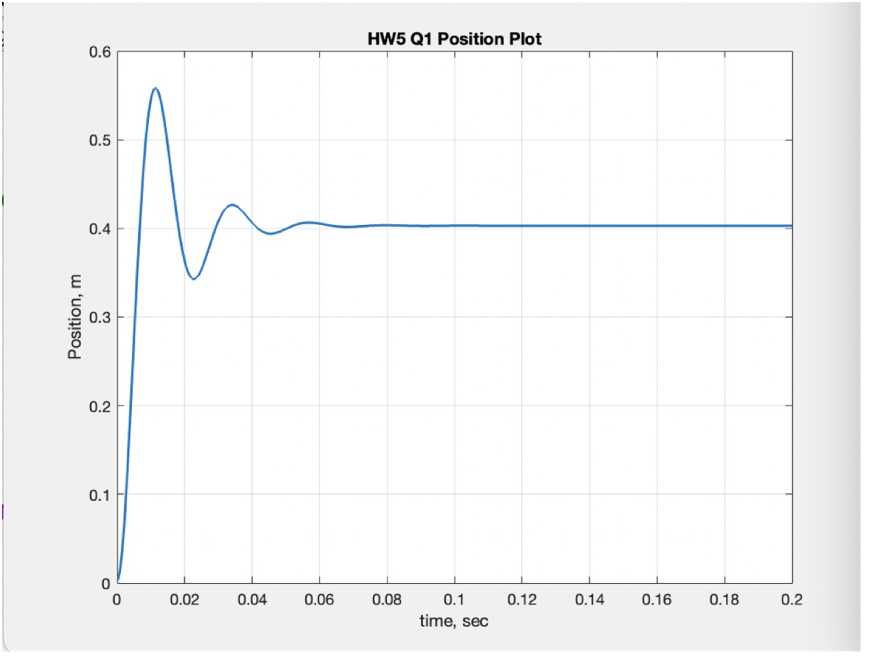
Position response settling at 0.4 m with a 1000 N external force — Position with a 1000 N external force applied.

Adding 1000 N of external force moves it to 0.4 m. The force dominates the electrical input completely, and the response rings out and settles in about 0.06 seconds.

DC shunt motor

Speed and current under load

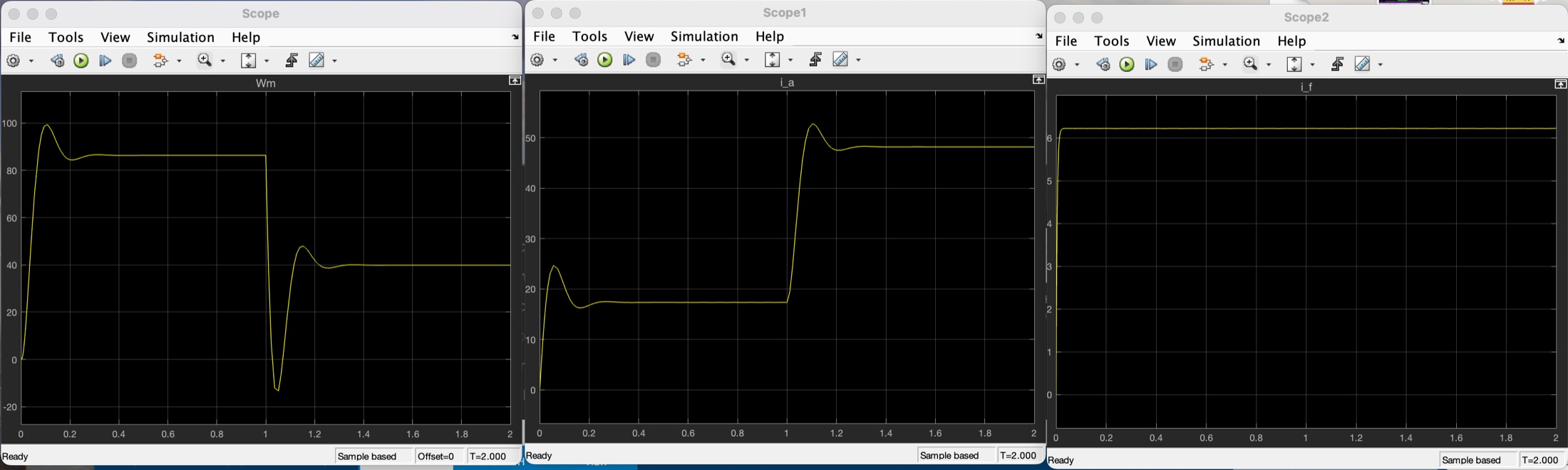
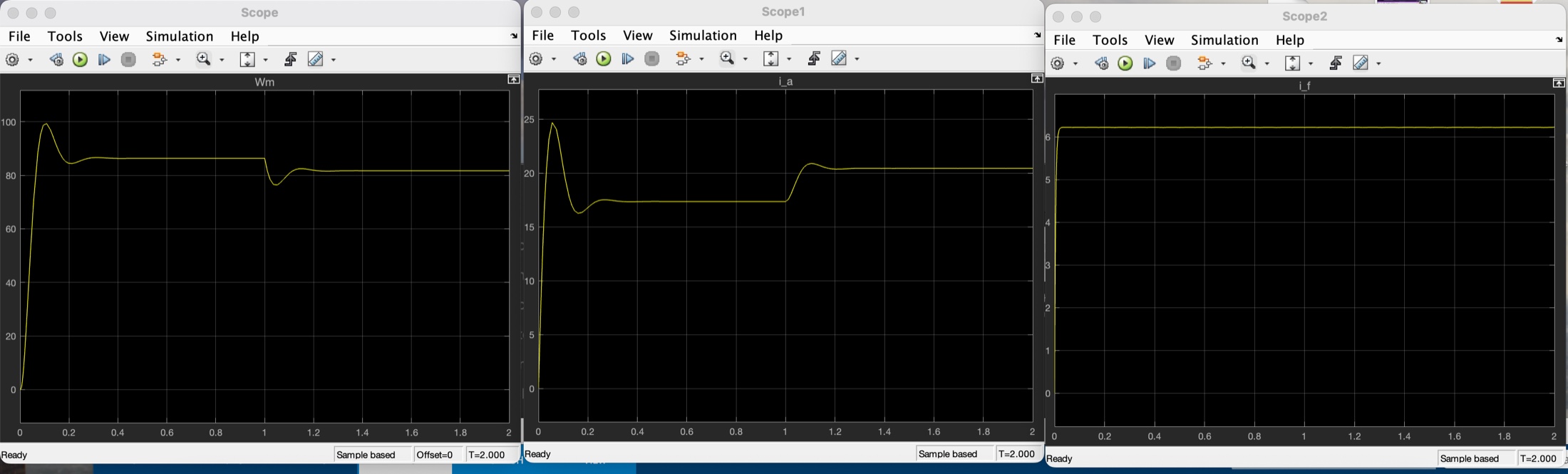
The load step lands at one second. Speed drops, current climbs to meet it.

Scopes for the motor with a 100 Nm load step — Load step to 100 Nm. Speed, armature current, field current.

Scopes for the motor with a 1000 Nm load step — Load step to 1000 Nm.

Load step	Settled speed	Armature current
0 → 100 Nm	~80 rpm	~22 A
0 → 1000 Nm	~40 rpm	~48 A

Field current stays flat in both cases, which is what makes it a shunt machine — the field winding sits across the same supply, so the load has no path to disturb it.

Inverted pendulum

Where it stops being stable

The input threshold sits at about u = 0.2.

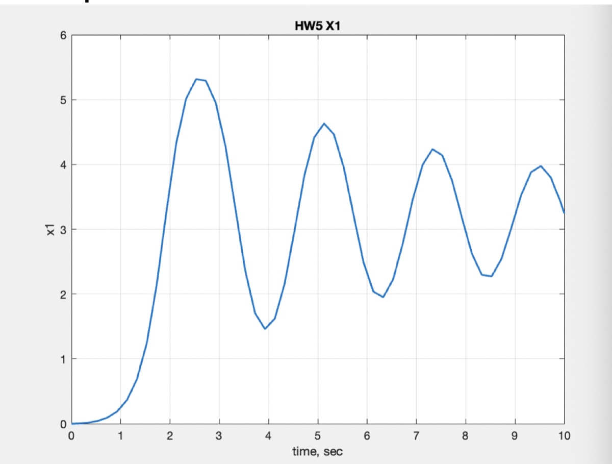
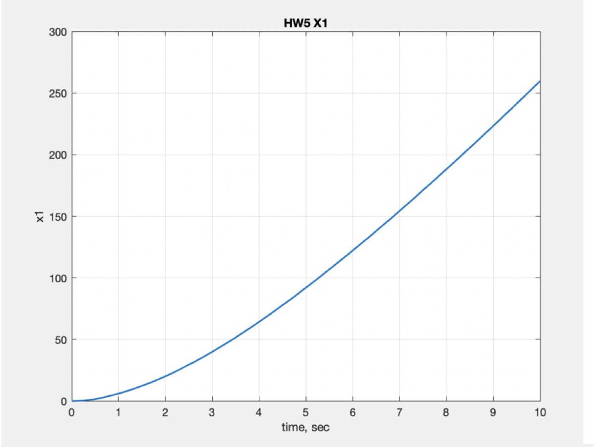
x1 oscillating around a constant value of about 3 at u = 0.01 — u = 0.01 — oscillates around 3.

x1 growing without bound at u = 2 — u = 2 — runs away.

Below that threshold x1 oscillates around a constant value. Above it the response climbs and does not come back.

MATLAB and Simulink. Coursework for ME 3360 at Ohio State, autumn 2024.